Introduction
splicer.js is a reactive computation library based on finite differencing.
Given a source domain \(A\), a target domain \(B\), and a pure function \(f: A \to B\), we maintain two variables \(x \in A\) and \(y \in B\) such that \(y = f(x)\) always holds. When \(x\) changes by some delta \(\Delta x\), we derive a delta propagator \(\Delta f\) such that:
\[ f(x + \Delta x) = f(x) + \Delta f(x, \Delta x) \]
This patches \(y\) directly - without rerunning \(f\) from scratch.
See the README for the full motivation and comparison with incremental computation and reactivity.
Research Material
This section collects papers and resources relevant to splicer.js's approach. The material is organized by topic: finite differencing (the core technique), general incremental computation (for contrast), differential dataflow (delta propagation applied to collections), and surveys.
Surveys
- Ramalingam & Reps, "A Categorized Bibliography on Incremental Computation" (1993)
- Comprehensive survey of the field up to 1993. Categorizes work into: value caching / memoization, static dependency analysis, dynamic dependency tracking, and finite differencing. Useful for understanding how the different approaches relate.
- ACM Digital Library
Incremental Computation
General incremental computation builds a dependency graph at runtime, traces which subcomputations read which inputs, and selectively re-executes stale nodes. Included here for contrast with the finite differencing approach.
Key works
-
Acar, "Self-Adjusting Computation" (PhD thesis, Carnegie Mellon, 2005)
- The foundational work on runtime dependency tracking for incremental computation. Programs are written normally; the runtime records a dynamic dependency graph and replays only the affected parts when inputs change.
- CMU Tech Report
-
Hammer, Phang, Hicks, Foster, "Adapton: Composable, Demand-Driven Incremental Computation" (PLDI 2014)
- Introduces lazy, demand-driven incremental computation. Unlike self-adjusting computation (which eagerly propagates changes), Adapton only re-evaluates nodes when their results are demanded. Composable - subcomputations can be independently incremental.
- ACM Digital Library
-
Acar, Blelloch, Harper, "Adaptive Functional Programming" (POPL 2002)
- Earlier work on the same theme. Introduces modifiables (mutable inputs) and the change propagation algorithm that re-executes only affected code.
- ACM Digital Library
Differential Dataflow
Delta propagation applied to dataflow systems. Instead of propagating values, these systems propagate collections of differences through a dataflow graph.
Key works
-
McSherry, Murray, Isaacs, Isard, "Differential Dataflow" (CIDR 2013)
- Operators consume and produce streams of differences (deltas) rather than full collections. Supports iterative computations. The key insight: if every operator can process differences, the entire pipeline becomes incremental without per-operator special-casing.
- CIDR Paper
-
Murray, McSherry, Isaacs, Isard, Barham, Abadi, "Naiad: A Timely Dataflow System" (SOSP 2013)
- The runtime system underlying differential dataflow. Introduces timely dataflow - a model that supports both streaming and iterative computation with consistent progress tracking.
- ACM Digital Library
Finite Differencing
The core technique behind splicer.js. The idea: given a program that computes \(f(x)\), systematically derive a maintenance program \(\Delta f\) that updates the result when \(x\) changes, without rerunning \(f\) from scratch.
Foundational
- Paige & Koenig, "Finite Differencing of Computable Expressions" (1982)
- The original paper. Introduces the idea of systematically deriving maintenance code from a program by computing "finite differences" of expressions - analogous to derivatives in calculus but for discrete program transformations.
- ACM Digital Library
Higher-order extensions
-
Cai, Giarrusso, Rendel, Ostermann, "A Theory of Changes for Higher-Order Languages - Incrementalizing Lambda-Calculi by Static Differentiation" (PLDI 2014)
- Formalizes delta propagation for higher-order functions. Introduces change structures (a type paired with a notion of delta) and program derivatives (given \(f\), mechanically derive its delta propagator \(\Delta f\)). The most directly relevant formalization of what splicer.js does.
- ACM Digital Library
-
Giarrusso, "Optimizing and Incrementalizing Higher-Order Collection Queries by AST Transformation" (PhD thesis, 2020)
- Extends the incremental lambda-calculus work toward practical use, with focus on collection operations. Covers both the theory and compilation strategies for deriving efficient delta propagators.
Notes
Reading notes corresponding to each research material section. These capture key takeaways, open questions, and how each paper relates to splicer.js.
A Categorized Bibliography on Incremental Computation
Ramalingam & Reps, 1993. ACM Digital Library.
See research material.
Important keywords:
- Incremental computation.
- Batch computation.
- Dynamization of static problems.
- Selective recomputation.
- Finite differencing.
Abstract
Small changes in the input to a computation often cause only small changes in the output. Rather than recomputing from scratch, we should be able to propagate only the delta. But until recently, I haven't known of a technique to do this efficently? Specifically, how do we transform a delta on the input to a delta on the output? How do we measure performance supposing we're taking this approach? The area of incremental computation was pretty much new to me, so I decided to read this survey to first have an overview of the field first.
This survey formalizes the problem raised above as follows: given \(f\) and input \(x\), keep \(f(x)\) up to date as \(x\) changes. An incremental algorithm takes batch input \(x\), batch output \(f(x)\), a change \(\Delta x\), and auxiliary information maintained across updates, and produces \(f(x + \Delta x)\).
The idea turns out to be everywhere. Similar notions of incremental computation arose in many fields but before this survey, little effort has been spent to unify these notions. This survey was intended to not only focus on the techniques within the programming language community, but also take a look in other areas as well.
The PL community cares about it for:
- Reactive language primitives (observables, signals, etc)
- Compiler optimization, especially in loops, in which changes between iterations can be small.
- Responsive dev tools, such as IDE-centric program analyzers/compilers should not re-do it from scratch every time the user edits a file.
However, there is a less well-known body of related work in algorithms:
- Dynamic graph problems
- Dynamization of static structures
- Databases (view maintenance)
- AI (truth maintenance)
- VLSI (incremental design-rule checking)
All working on variants of the same underlying problem.
Introduction
Small updates in input usually cause small changes in output. Therefore, the intuition is that it's more efficient to compute the changes it takes to go from the previous output to the new output, rather than recompute the output from scratch.
The authors survey this idea across multiple fields, deliberately bridging between programming languages research and work in algorithms, AI, databases, and VLSI.
"Because small changes in the input to a computation often cause only small changes in the output, the challenge is to compute the new output incrementally by updating parts of the old output, rather than by recomputing the entire output from scratch."
"The goal is to make use of the solution to one problem instance to find the solution to a 'nearby' problem instance."
"In so doing, the goal was to expose ties between the ideas on incremental computation that developed out of research on programming languages and programming tools, and ideas that have been developed by researchers in other areas."
The authors identify four areas where PL people care about incrementality:
- Reactive language primitives: baking reactivity into languages (observables, signals, etc).
- Compiler optimization: using incrementality as a compiler trick, e.g. loop optimization where changes between iterations are small.
- Responsive dev tools: incremental parsing, type-checking, etc. This is what modern LSPs and IDEs do. Don't re-analyze the whole file on every keystroke.
- Compilers and tooling: the practical realization of the first three.
But the survey also points to a less well-known body of work outside PL that I think is just as important:
- Comparison criteria: how do you even measure whether an incremental algorithm is "good"? Standard batch complexity doesn't cut it.
- General principles: things like dynamization of static problems. I think of this as foundational formulation/modeling.
- Problem-specific results: results on individual incremental problems that might reveal new general principles.
Assessment of Incremental Algorithms
Computational Complexity
This is the "how do you measure it" section. Standard asymptotic analysis (big-O on total input size) doesn't work well for incremental problems. Under those criteria, an incremental algorithm and a full recomputation can look the same, or worse, the batch start-over can be deemed "optimal" for some incremental problems. That feels wrong.
The survey lays out several alternative criteria that make more sense:
- Direct comparison: just compare against the batch start-over algorithm directly.
- Amortized-cost analysis: average the cost over a worst-case sequence of operations. This is closer to how I'd intuitively think about incremental performance.
- Competitiveness: how much worse does an online algorithm (no future knowledge) do vs an optimal offline algorithm (perfect future knowledge), assuming an adversary picks the worst-case sequence? The competitive ratio is max cost(online) / cost(offline); lower is better, 1 is optimal. Interestingly, randomized online algorithms can beat the best deterministic ones, because the randomness limits what the adversary can exploit.
- Probabilistic analysis: average-case performance under random inputs, as opposed to worst-case.
- Incremental relative lower bounds: proving that for certain problems, no incremental algorithm can do better than batch start-over by more than some factor.
- Reductions between problems: showing one incremental problem is at least as hard as another, transferring bounds across problems.
- Boundedness: this one is interesting. Instead of cost as a function of total input size, measure cost as a function of \(|\Delta x| + |\Delta f(x)|\). An incremental algorithm is "bounded" if its update time depends only on the size of the change, never on the size of the full input. I think this is the most natural way to think about incrementality: ideally, if the change is small, the work should be small, regardless of how big the whole thing is.
Measurements of Actual Performance
Few experimental evaluations of incremental algorithms exist. But the ones that do suggest something surprising: theoretically "bad" incremental algorithms can still perform well in practice. Real workloads may not hit worst cases. So the theoretical criteria above don't tell the whole story.
Data-Structure Update Problems
Incremental Annotations on Graphs/Trees
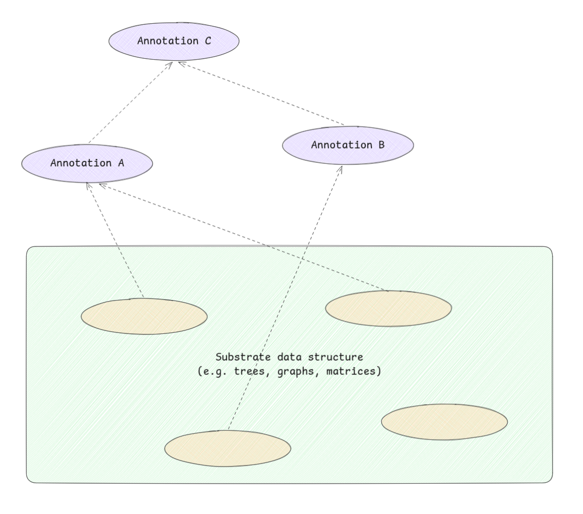
This section covers a specific class of problem that I think is very relevant to what I'm building. The setup is:
- You have a "substrate" data structure \(x\), a tree, graph, matrix, whatever. This is the thing that changes.
- \(f(x)\) maps the substrate's state to some "annotation" on it. Think of annotating an AST with type information or symbol resolution.
- The problem: keep those annotations up to date as the substrate changes.
Annotations can depend on other annotations too, so changes can cascade.
The survey identifies three approaches:
- Selective recomputation: figure out which annotations are affected by a substrate change, then recompute only those.
- A recomputed annotation if not changes may not need to trigger recomputation of further dependent annotations.
- This is the approach behind:
- Incremental updating of attributed derivation trees/augmented ASTs.
- Incremental circuit-annotation problem.
- Incremental data-flow analysis.
- Path problems (e.g. shortest paths) in graphs.
- At Holistics, the AML compiler mirrors salsa, presumably using this pattern also.
- Differential updating: instead of recomputing affected annotations from scratch, compute the difference to apply. Related to database view maintenance and the INC language.
- Other incremental expression-evaluation algorithms:
- Function caching.
- Incremental reduction in the lambda calculus.
- Dynamic expression trees.
Other Dynamic Graph Problems
Maintaining:
- Graph properties (connectivity, transitive closure
- Minimum spanning trees.
- Planarity.
under edge insertions and deletions.
I'm not entirely sure whether "edge" here always means the lines between nodes or sometimes refers to leaf nodes?
The work covers a wide range, from Even & Shiloach's early edge-deletion problem (1981) through to Eppstein et al's sparsification technique (1992).
Dynamization of Static Data Structures
This is a general methodology for transforming a static data structure into a dynamic one.
What does "static" mean here exactly? I think it means a structure that's built from scratch given the inputs, no support for incremental updates baked in.
Finite Differencing
Finite differencing is about automatically deriving incremental maintenance logic from batch definitions. You write the batch computation, and the technique derives how to update the output when the input changes. This is exactly what splicer.js is looking for.
The foundational paper is Paige & Koenig (1982) on finite differencing of computable expressions. Earlier work by Earley on high-level iterators and by Fong & Ullman on induction variables laid the groundwork.
Incremental Formal Systems
This section covers incrementalizing formal operations: reduction, parsing, deduction, constraint solving. I think of these as generic-but-also-specific techniques, each one applies a general incremental idea to a particular formal system.
- Incremental reduction: goes back to Lombardi & Raphael's early work on Lisp as a language for incremental computation (1964). More recent work includes partial evaluation (Sundaresh & Hudak) and incremental reduction in the lambda calculus (Field & Teitelbaum).
- Incremental parsing: how do you re-parse a file when only a small part changed? Work here includes augmenting parsers for incrementality (Ghezzi & Mandrioli), building "friendly" parsers (Jalili & Gallier), and even incremental parsing without a parser (Kaiser & Kant).
- Truth maintenance: from AI, starting with Doyle's foundational truth maintenance system (1979). The problem: when your assumptions change, how do you maintain consistency of all derived beliefs? de Kleer extended this with assumption-based TMS.
- Incremental deduction: rule support in Prolog, unification in many-sorted algebras, deriving incremental implementations from algebraic specifications.
- Incremental constraint solving: constraint satisfaction for graphical interfaces (Vander Zanden), incremental constraint solvers (Freeman-Benson et al).
Applications, Frameworks, and Related Problems
The remaining sections cover more applied work. These feel less central to what I'm after, but worth noting:
-
Special-purpose algorithms: domain-specific applications, including incremental compilation (DICE, Magpie), smart recompilation (Tichy), interactive document composition (JANUS), VLSI layout (Magic). These adapt incremental ideas to fairly niche fields.
-
Implementation frameworks: actual systems that enable incremental computation. VisiCalc (the original spreadsheet!) is listed here, along with the Synthesizer Generator, CENTAUR, PSG, Pan, and Alphonse. Also includes Cai & Paige's SETL-family work on binding performance at language design time.
-
Related problems: problems with similar structure, such as sensitivity analysis in linear network optimization, parametric maximum flow, continuous execution (Visiprog).
Verdict
This survey draws bridges between PL and other fields that all use incremental ideas without necessarily talking to each other. It's from 1993, so it misses the modern reactive/FRP wave, but the foundations are all here. The section on finite differencing is the most relevant to splicer.js.
References
Assessment of Incremental Algorithms
| Authors | Year | Title | Venue |
|---|---|---|---|
| Yellin, Strom | 1991 | INC: A language for incremental computations | ACM TOPLAS |
| Sleator, Tarjan | 1983 | A data structure for dynamic trees | J Computer and System Sciences |
| Tarjan | 1985 | Amortized computational complexity | SIAM J Algebraic Discrete Methods |
| Sleator, Tarjan | 1985 | Amortized efficiency of list update and paging rules | CACM |
| McGeoch, Sleator (eds) | 1992 | On-Line Algorithms | AMS |
| Karp | 1992 | On-line algorithms versus off-line algorithms: How much is it worth to know the future? | IFIP |
| Lomchard et al | 1992 | Dynamic algorithms in D E Knuth's model: A probabilistic analysis | TCS |
| Berman, Paull, Ryder | 1990 | Proving relative lower bounds for incremental algorithms | Acta Informatica |
| Reif | 1987 | A topological approach to dynamic graph connectivity | IPL |
| Reps, Teitelbaum, Demers | 1983 | Incremental context-dependent analysis for language-based editors | ACM TOPLAS |
| Alpern et al | 1990 | Incremental evaluation of computational circuits | ACM-SIAM SODA |
| Ramalingam, Reps | 1991-92 | On the computational complexity of incremental algorithms | UW-Madison TR |
| Dionne | 1978 | Etude et extension d'un algorithme de Marche | INFOR |
| Taylor, Ousterhout | 1984 | Magic's incremental design-rule checker | DAC |
| Scott, Ousterhout | 1984 | Plowing: Interactive stretching and compaction in Magic | DAC |
| Ryder, Landi, Pande | 1990 | Profiling an incremental data flow analysis algorithm | IEEE Trans. Software Eng. |
| Harrison, Munson | 1991 | Numbering document components | Electronic Publishing |
Selective Recomputation
| Authors | Year | Title | Venue |
|---|---|---|---|
| Demers, Reps, Teitelbaum | 1981 | Incremental evaluation for attribute grammars with application to syntax-directed editors | POPL |
| Reps | 1982 | Optimal-time incremental semantic analysis for syntax-directed editors | POPL |
| Reps, Teitelbaum, Demers | 1983 | Incremental context-dependent analysis for language-based editors | ACM TOPLAS |
| Reps | 1984 | Generating Language-Based Environments | MIT Press |
| Yeh | 1983 | On incremental evaluation of ordered attributed grammars | BIT |
| Jones, Simon | 1986 | Hierarchical VLSI design systems based on attribute grammars | POPL |
| Reps, Marceau, Teitelbaum | 1986 | Remote attribute updating for language-based editors | POPL |
| Hoover, Teitelbaum | 1986 | Efficient incremental evaluation of aggregate values in attribute grammars | SIGPLAN Compiler Construction |
| Hoover | 1987 | Incremental graph evaluation | Cornell PhD |
| Kaiser | 1989 | Incremental dynamic semantics for language-based programming environments | ACM TOPLAS |
| Teitelbaum, Chapman | 1990 | Higher-order attribute grammars and editing environments | PLDI |
| Zaring | 1990 | Parallel evaluation in attribute grammar based systems | Cornell PhD |
| Alpern et al | 1990 | Incremental evaluation of computational circuits | ACM-SIAM SODA |
| Ramalingam, Reps | 1991-92 | On the computational complexity of incremental algorithms | UW-Madison TR |
| Rosen | 1981 | Linear cost is sometimes quadratic | POPL |
| Ryder | 1982 | Incremental data flow analysis based on a unified model of elimination algorithms | Rutgers PhD |
| Zadeck | 1983-84 | Incremental data flow analysis in a structured program editor | Rice PhD / SIGPLAN Compiler Construction |
| Cooper, Kennedy | 1986 | The impact of interprocedural analysis and optimization in the Rn programming environment | ACM TOPLAS |
| Burke; Burke, Ryder | 1987 | Interval-based and iterative incremental data-flow analysis | IBM TR |
| Carroll, Ryder | 1988 | Incremental data flow update via attribute and dominator updates | POPL |
| Ryder, Paull | 1988 | Incremental data flow analysis algorithms | ACM TOPLAS |
| Marlowe; Marlowe, Ryder | 1989-90 | Efficient hybrid algorithm for incremental data flow analysis | Rutgers PhD / POPL |
| Murchland 1967 ... Ramalingam, Reps 1992 | 1967-92 | Maintaining shortest distances in graphs | Various |
Differential Updating
| Authors | Year | Title | Venue |
|---|---|---|---|
| Koenig, Paige | 1981 | A transformational framework for the automatic control of derived data | VLDB |
| Shmueli, Itai | 1984 | Maintenance of views | ACM SIGMOD |
| Horwitz; Horwitz, Teitelbaum | 1985-86 | Generating editing environments based on relations and attributes | Cornell PhD / ACM TOPLAS |
| Yellin, Strom | 1991 | INC: A language for incremental computations | ACM TOPLAS |
Other Incremental Expression-Evaluation
| Authors | Year | Title | Venue |
|---|---|---|---|
| Pugh; Pugh, Teitelbaum | 1988-89 | Incremental computation via function caching | Cornell PhD / POPL |
| Field, Teitelbaum; Field | 1990-91 | Incremental reduction in the lambda calculus | ACM Lisp/FP / Cornell PhD |
| Cohen, Tamassia | 1991 | Dynamic expression trees and their applications | ACM-SIAM SODA |
Dynamic Graph Problems
| Authors | Year | Title | Venue |
|---|---|---|---|
| Cheston | 1976 | Incremental algorithms in graph theory | U Toronto PhD |
| Even, Shiloach | 1981 | An on-line edge-deletion problem | J ACM |
| Frederickson | 1985 | Data structures for on-line updating of minimum spanning trees | SIAM J Computing |
| Italiano | 1986 | Amortized efficiency of a path retrieval data structure | TCS |
| Reif | 1987 | A topological approach to dynamic graph connectivity | IPL |
| La Poutre, van Leeuwen | 1988 | Maintenance of transitive closures and transitive reductions of graphs | WG |
| Italiano | 1988 | Finding paths and deleting edges in directed acyclic graphs | IPL |
| Yellin | 1988 | A dynamic transitive closure algorithm | IBM TR |
| Di Battista, Tamassia | 1989 | Incremental planarity testing | FOCS |
| Buchsbaum, Kanellakis, Vitter | 1990 | A data structure for arc insertion and regular path finding | ACM-SIAM SODA |
| Yannakakis | 1990 | Graph-theoretic methods in database theory | PODS |
| Frederickson | 1991 | Ambivalent data structures for dynamic 2-edge-connectivity and k smallest spanning trees | FOCS |
| Galil, Italiano | 1991 | Fully dynamic algorithms for edge-connectivity problems | STOC |
| Kanevsky et al | 1991 | On-line maintenance of the four-connected components of a graph | FOCS |
| La Poutre | 1992 | Maintenance of triconnected components of graphs | ICALP |
| Eppstein, Galil, Italiano, Nissenzweig | 1992 | Sparsification: A technique for speeding up dynamic graph algorithms | FOCS |
Dynamization of Static Data Structures
| Authors | Year | Title | Venue |
|---|---|---|---|
| Bentley | 1979 | Decomposable searching problems | IPL |
| Bentley, Saxe | 1980 | Decomposable searching problems I: Static-to-dynamic transformations | J Algorithms |
| Overmars | 1983 | The Design of Dynamic Data Structures | Springer LNCS |
| Mehlhorn | 1984 | Data Structures and Algorithms 3: Multi-Dimensional Searching and Computational Geometry | Springer |
| Eppstein, Galil, Italiano, Nissenzweig | 1992 | Sparsification: A technique for speeding up dynamic graph algorithms | FOCS |
Finite Differencing
| Authors | Year | Title | Venue |
|---|---|---|---|
| Earley | 1974-76 | High-level operations in automatic programming / High-level iterators | SIGPLAN VHL / J Computer Languages |
| Fong, Ullman; Fong | 1976-79 | Induction variables / Common subexpressions / Inductively computable constructs in VHL languages | POPL |
| Paige, Koenig | 1982 | Finite differencing of computable expressions | ACM TOPLAS |
| Goldberg, Paige | 1984 | Stream processing | ACM Lisp/FP |
| Paige | 1986 | Programming with invariants | IEEE Software |
Incremental Formal Systems
| Authors | Year | Title | Venue |
|---|---|---|---|
| Lombardi, Raphael; Lombardi | 1964-67 | Lisp as the language for an incremental computer / Incremental computation | MIT Press / Advances in Computers |
| Sundaresh, Hudak; Sundaresh | 1991 | Incremental computation via partial evaluation | POPL / Yale PhD |
| Field, Teitelbaum; Field | 1990-91 | Incremental reduction in the lambda calculus | ACM Lisp/FP / Cornell PhD |
| MacLennan | 1986-87 | A calculus of functional differences and integrals | Naval Postgraduate School TR |
| Ghezzi, Mandrioli | 1979-80 | Incremental parsing / Augmenting parsers to support incrementality | ACM TOPLAS / J ACM |
| Wegman | 1980 | Parsing for structural editors | FOCS |
| Jalili, Gallier | 1982 | Building friendly parsers | POPL |
| Kaiser, Kant | 1985 | Incremental parsing without a parser | J Systems and Software |
| Doyle | 1979 | A truth maintenance system | Artificial Intelligence |
| de Kleer | 1986 | An assumption-based TMS / Extending the ATMS / Problem solving with the ATMS | Artificial Intelligence |
| McAllister | 1990 | Truth maintenance | AAAI |
| Shmueli, Tsur, Zfira | 1984 | Rule support in Prolog | |
| Mannila, Ukkonen | 1988 | Time parameter and arbitrary deletions in the set union problem | SWAT |
| Snelting, Henhapl | 1986 | Unification in many-sorted algebras for incremental semantic analysis | POPL |
| Ballance; Ballance, Graham | 1989-91 | Syntactic/semantic checking and incremental consistency maintenance | UC Berkeley PhD / ICLP |
| van der Meulen | 1990 | Deriving incremental implementations from algebraic specifications | CWI TR |
| Vander Zanden | 1988 | Incremental constraint satisfaction and its application to graphical interfaces | Cornell PhD |
| Freeman-Benson, Maloney, Borning | 1990 | An incremental constraint solver | CACM |
Special-Purpose Algorithms
| Authors | Year | Title | Venue |
|---|---|---|---|
| Fritzson | 1984 | Preliminary experience from the DICE system | ACM SIGPLAN/SIGSOFT |
| Schwartz, Delisle, Begwani | 1984 | Incremental compilation in Magpie | SIGPLAN Compiler Construction |
| Tichy | 1986 | Smart recompilation | ACM TOPLAS |
| Schwanke, Kaiser | 1988 | Smarter recompilation | ACM TOPLAS |
| Cooper, Kennedy | 1986 | The impact of interprocedural analysis and optimization in the Rn programming environment | ACM TOPLAS |
| Burke, Torczon | Interprocedural optimization: Eliminating unnecessary recompilation | ACM TOPLAS | |
| Chamberlain et al | 1981-87 | JANUS: An interactive system for document composition / Document convergence | ACM SIGPLAN / IBM Systems J |
| Chen, Harrison; Harrison, Munson | 1988-91 | Multiple representation document development / Integrated bibliography / Numbering document components | IEEE Computer / Electronic Publishing |
| Brooks | 1988 | A two-view document editor with user-definable document structure | DEC Systems Research Center TR |
| Ousterhout et al | 1984 | Magic: A VLSI layout system | DAC |
| Taylor, Ousterhout | 1984 | Magic's incremental design-rule checker | DAC |
| Scott, Ousterhout | 1984 | Plowing: Interactive stretching and compaction in Magic | DAC |
Implementation Frameworks
| Authors | Year | Title | Venue |
|---|---|---|---|
| Bricklin, Frankston | 1979 | VisiCalc | Personal Software Inc |
| Alpern et al | 1989 | Graph attribution as a specification paradigm | ACM SIGPLAN/SIGSOFT |
| Borning | 1979 | ThingLab: A constraint-oriented simulation laboratory | Stanford PhD / Xerox PARC |
| Konopasek, Jayaraman | 1984 | The TK!Solver Book | Osborne/McGraw-Hill |
| Reps, Teitelbaum | 1988 | The Synthesizer Generator | Springer |
| Borras et al | 1988 | CENTAUR: The system | ACM SIGPLAN/SIGSOFT |
| Bahlke, Snelting | 1986 | The PSG system: From formal language definitions to interactive programming environments | ACM TOPLAS |
| Ballance, Graham, Van De Vanter | 1992 | The Pan language-based editing system | ACM TOSEM |
| Paige, Koenig | 1982 | Finite differencing of computable expressions | ACM TOPLAS |
| Cai, Paige | 1987-91 | Binding performance at language design time / Program derivation by fixed point computation / Languages polynomial in input+output | POPL / Science of Computer Programming / AMAST |
| Hoover | 1992 | Alphonse: Incremental computation as a programming abstraction | PLDI |
Related Problems
| Authors | Year | Title | Venue |
|---|---|---|---|
| Bertsekas | 1991 | Linear Network Optimization: Algorithms and Codes | MIT Press |
| Gallo, Grigoriadis, Tarjan | 1989 | A fast parametric maximum flow algorithm and applications | SIAM J Computing |
| Henderson, Weiser | 1985 | Continuous execution: The Visiprog environment | IEEE ICSE |
Acar - Self-Adjusting Computation (PhD thesis, 2005)
See research material.
(TODO)
Hammer et al. - Adapton (PLDI 2014)
See research material.
(TODO)
Acar, Blelloch, Harper - Adaptive Functional Programming (POPL 2002)
See research material.
(TODO)
McSherry et al. - Differential Dataflow (CIDR 2013)
See research material.
(TODO)
Murray et al. - Naiad (SOSP 2013)
See research material.
(TODO)
Finite Differencing of Computable Expressions
Paige & Koenig, 1982. ACM Digital Library
See research material.
Important keywords:
- Program optimization.
- Finite differencing.
- Strength reduction.
- Iterator inversion.
- Formal differentiation.
Abstract
- The paper frames finite differencing as a "program optimization method" that generalizes strength reduction (replacing expensive operations with cheaper ones).
- Finite differencing also enables efficient implementation of other program transformations, e.g. "iterator inversion."
- The formalization works by composing basic semantics-preserving transformations.
Introduction
- Paige developed "formal differentiation" as a global program optimization that captures a recurring pattern: replacing repeated costly calculations with inexpensive incremental updates.
- Applied to high-level but inefficient problem statements, the transformed algorithms become more complex but more efficient. The method generalizes Cocke's strength reduction and provides a framework for Earley's "iterator inversion."
- The authors prefer "finite differencing" over "formal differentiation" to place it in proper historical context: a link to 16th-century finite difference techniques invented to reduce labor in calculations.
- Language-independent algorithms to implement finite differencing were devised. Most useful for very high-level languages, so set-theoretic finite differencing was the focus.
What makes finite differencing stand out:
- Flexible: works at very high-level or low-level language levels.
- Can quickly converge from high-level inefficient form to a much lower-level efficient implementation.
- Can be implemented systematically, following a well-known methodology.
- Can be shown to yield asymptotic speedup, not just hoped-for improvement.
Historical Perspective
This section walks us through the progression of history that leads to the author's idea.
Finite differencing as a Mathematical Method
Henry Briggs (16th century) used finite differencing to tabulate polynomial values. The problem was that: given a polynomial \(p(x)\), generate an indefinite evenly spaced values \(p(x_0)\), \(p(x_0 + h)\), \(p(x_0 + 2h)\), ... without evaluating the polynomial from scratch each time.
The key observation, if \(p(x)\) has degree \(n\)), then, define difference polynomials as follows:
- \(p_0(x) = p(x)\), which has degree \(n\).
- \(p_1(x) = p_0(x + h) - p_0(x)\), which has degree \(n - 1\).
- ...
- \(p_n(x) = p_{n-1}(x+h) - p_{n-1}(x)\), which has a degree \(0\). In other words, \(p_n\) is constant.
Example with \(p(x) = x^2\), \(h = 1\):
| \(x\) | \(p(x) = x^2\) | 1st difference | 2nd difference |
|---|---|---|---|
| 0 | 0 | ||
| 1 | 1 | 1 | |
| 2 | 4 | 3 | 2 |
| 3 | 9 | 5 | 2 |
| 4 | 16 | 7 | 2 |
| 5 | 25 | 9 | 2 |
The finite differencing method is as follows:
-
Compute initial values:
- \(t(1) = p(x_0)\).
- \(t(2) = p_1(x_0)\).
- ...
- \(t(n+1) = p_n(x_0)\).
-
Then iterate repeatedly until all desired values have been computed:
print x, t(1);
t(1) := t(1) + t(2);
t(2) := t(2) + t(3);
...
t(n) := t(n) + t(n + 1);
x := x + h;
Loop invariant, at iteration \(i\):
- \(t(1) = p(x_i)\).
- \(t(2) = p_1(x_i)\).
- ...
- \(t(n) = p_{n-1}(x_i)\).
- \(t(n+1) = p_n(x_i)\).
Note that each loop iteration need not update \(t(n + 1)\) as \(t(n+1)\) is constant. Therefore, each iteration is just \(n\) additions (one per \(t(1)\), \(t(2)\), ..., \(t(n)\)), instead of \(n\) additions and \(n\) multiplications as in Horner's rule.
Babbage's difference engine was built to automate step 2. Note that step 2 is the same regardless of the exact polynomials, so it can be automated. Digital computers through WWII were designed for the same task: finite differencing for gunnery tables.
There's something intriguing about the idea that the earliest computers were incremental computation machines.
Reduction in Operator Strength
John Cocke (1960s) discovered "reduction in operator strength", a program optimization method, that highlighted the impact of finite differencing methods in the speedup of FORTRAN programs.
Before delving into the illustrative example, I researched a few concepts in the area of program optimization. Disclaimer, I don't have an expertise in this area at the time of writing.
- A strongly connected component in a directed graph is a maximal subgraph where every vertex is reachable from every other vertex within that subgraph.
- Code block: A sequence of instructions that has only one entry point and one exit point.
- Program region: Possibly a directed subgraph of code blocks.
- Strongly connected program region: I suppose that strongly connected means as it is in graph theory. This means a maximal subgraph of code block in which starting from one code block, there's a possible path to any other code blocks.
Illustrative example:
-
Suppose the following situation:
- A strongly connected program region \(R\).
- An expression \(i * c \) occurs in \(R\), in which \(c\) is a region constant (supposedly a variable that cannot change within \(R\)) and \(i\) is defined before every entry to \(R\), while \(i\) is not.
- \(i * c\) cannot be moved out of \(R\) because there are redefinitions to \(i\).
- All redefinitions to \(i\) within \(R\) are of the form \(i = i \pm \text{delta}\), \(\text{delta}\) is also a region constant.
-
A concrete version of the above situation:
const int c = 10; // region constant `c` const int delta = 1; // region constant `delta` int sum = 0; for (int i = 0; i <= 100; i = i + delta) { sum += i * c; // expression in question } -
The question: How do we move all calulations of \(i * c\) out of \(R\)?
-
Idea:
- Insert an initial assignment \(T = i * c\), \(T\) is a compiler-generated variable, prior to any entry points of \(R\).
- Before each redefinition \(i = i \pm \text{delta}\), we can replace it with a redefinition \(T \pm \text{delta} * c\).
- Because \(\text{delta}\) and \(c\) are region constants, \(\text{delta} * c\) is invariant. Thus, it can be moved out of \(R\).
- Now replace all uses of \(i * c\) with uses of \(T\).
-
Impact: All \(i * c\) are replaced with \(T\), other operations stay roughly the same, except for the additional initial computations.
Cocke's strength reduction technique is powerful enough that it can transform repeated polynomial calculations according to Horner's rule into one that is essentially Briggs' finite difference method. Note that Cocke's technique doesn't even treat polynomials specially, but manages to converge into a technique esstentially as finite differencing. This shows that inherently, finite differencing works due to properties of elementary operations, not exclusive properties of polynomials (say, the degree observation above).
These properties are the distributive and associative laws for sums and products.
Extensions
- Cocke and Schwarts later extended this strength reduction idea (also called as finite differencing by the authors) to all arithmetic operations having appropriate distributive properties.
- Earley suggest applying finite differencing in a set theoretic context.
- Fong and Ullman later proved that Earley's method can improve the asymptotic behavior of an algorithm. A theoretical characterization could then be developed to determine when this technique can be applied.
- Finite differencing was generalized further by Paige to allow its application in many type of expressions with various operations and data types.
Definitions and Notations
Language
Finite differencing is language-agnostic, but SETL is used in this paper for illustrative purposes.
SETL seems to allow the programmer to work on many levels of abstractions, ranging from concrete FORTRAN to set-theory level.
Data types in SETL: heterogeneous tuples, sets and maps.
- Tuples: Ordered from first to the last component.
- Sets: Unordered and can only contain unique elements.
- Maps: Sets of pairs \(([x, y]\)), each associating a domain value \(x\) to a range value \(y\).
Primitive operations:
| Primitive operations | Remarks |
|---|---|
| \(x + y\) | Addition for integers/reals. Union for sets. Concatenation for strings and tuples. |
| \(x - y\) | Subtraction for integers/reals. Difference for sets. |
| \(x * y\) | Multiplication for integers/reals. Intersection for sets. |
| \(x \in y\), \(x \notin y\) | Tests membership in a set or tuple. |
| \(#x\) | Returns the cardinality of a set, or the length of a tuple or string. |
| arb \(x\) | Picks an arbitrary element from set \(x\). arb \(\{\}\) yields the undefined atom om. |
| \(x\) incs \(y\) | Returns whether set \(x\) includes set \(y\). |
| \(x\) with \(y\) | Equivalent to \(x + \{y\}\) if \(x\) is a set, or \(x + [y]\) if \(x\) is a tuple. |
| \(x\) less \(y\) | Equivalent to \(x - \{y\}\). |
| \(\{x, y, \ldots\}\) | Set literal. |
| \([x, y, \ldots]\) | Tuple literal. |
-
C-like convention: \(x := x \text{op} \textit{exp}\) can be abbreviated as \(x \text{op}:= \text{exp}\).
-
APL reduction operation: \(\text{binop}/Q\), which folds a binary associative operator \(\text{binop}\) over all elements of a set or tuple \(Q\).
-
Powerful iterators: Allow constrained search through sets and tuples.
- Can be combined.
- Can be used as arguments to various iterative operations.
-
The most basic example to illustrate iterators is the forall loop (\(\forall\)-loop):
(∀x ∈ s | x mod 2 = 0)
  block(x)
end ∀;
This executes
blockfor each even number ins.Internal implementation:
- Iterate through
sselecting each value without repetition into the bound variablex. - Execute the predicate.
- Run the block when it holds.
If
sis a set, iteration order is unspecified; ifsis a tuple, iteration is from first to last component. - Iterate through
-
forall loops can implement many high-level iterator-involving expressions:
- Set former: Computes a subset satisfying a predicate. For example, \(\{x \in s \mid x \bmod 2 \neq 0\}\) gives all odd elements of \(s\). A variant \(\{x^2 : x \in s \mid x \bmod 2 \neq 0\}\) gives the set of squares of odd elements.
-
Range specifications: \([2 .. n-1]\) produces a tuple \([2, 3, \ldots, n-1]\). \(\{1, 3 .. 11\}\) produces all odd numbers from 1 to 11.
-
Bounded existential and universal quantifiers: A universal quantifier \(\forall j \in [2..n-1] \mid n \bmod j \neq 0\) tests primality. If it evaluates to false, \(j\) is assigned a witness as a side effect.
-
Map retrieval comes in three forms:
- \(f(a)\): Function application. Returns om if \(a\) is not in the domain or \(f\) is multivalued at \(a\).
- \(f\{a\}\): Image set of \(\{a\}\) under \(f\). Returns \(\{\}\) if \(a\) is not in the domain.
- \(f[S]\): Image of set \(S\) under \(f\), equivalent to \(+/\{f(a) : a \in S\}\).
-
Map modification via indexed assignment:
- \(f(a) := \textbf{om}\) removes \(a\) from the domain.
- \(f(a) := z\) first removes \(a\), then adds the pair \([a, z]\).
- \(f\{a\} \mathrel{+}:= \text{delta}\) modifies the image set at a domain point.
So map here is like a relation.
-
\(n\)-parameter maps are sets of pairs whose first component is an \(n\)-tuple. Notational shorthand: \(f(x, y, z)\) abbreviates \(f([x, y, z])\).
-
SETL uses copy value semantics, as in mathematics.
Verification
The authors extend SETL with two annotation statements for verification purposes:
- assume cond: A no-op during execution; marks a condition that is expected to hold.
- assert cond: Also a no-op; marks a condition that must hold.
An encounter with either statement is satisfied if the condition holds at that point.
An execution (not a program) is valid if:
- Whenever an unsatisfied assert encounter occurs, it was preceded by an unsatisfied assume encounter.
- Whenever all assume encounters are satisfied, execution terminates normally.
A program is valid if all possible executions are valid. The domain of a valid program \(P\) is the set of inputs for which every assumption encounter is satisfied.
Every program includes output assertions at normal exit points. A transformation \(T\) is:
- Validity preserving if \(T(P)\) preserves output assertions and remains valid whenever \(P\) is valid.
- Semantics preserving if additionally the domain of \(T(P)\) includes the domain of \(P\).
These notions also apply to single-entry, single-exit code blocks: replacing block \(B\) with \(B'\) is validity/semantics preserving when the same conditions hold within the enclosing program.
An achieve statement achieve E = f(x1, ..., xn) has the same semantics as an assignment E := f(x1, ..., xn).
Complexity
A way to measure expected efficiency is necessary to demonstrate finite differencing resulting in program speedup.
The authors adopted a heuristic complexity measure. This is supported by SETL runtime's storage structures.
The complexity model is based on SETL's runtime:
- Sets are expandable hash tables (unit-time membership test, linear-time full scan).
- Maps use hash tables for domains with fast access to range elements via domain elements.
| Operation | Estimated cost |
|---|---|
| \(s\) with:= \(x\) | \(O(1)\) * |
| \(s\) less:= \(x\) | \(O(1)\) * |
| \(x \in s\) | \(O(1)\) |
| \(s +\!:= \text{delta}\) | \(O(\#\text{delta})\) * |
| \(f(x) := y\) | \(O(1)\) * |
| \(f(x_1, \ldots, x_n)\) | \(O(n)\) |
| \((\forall x \in s)\) Block(\(x\)) \(\textbf{end}\ \forall\) | \(O(\#s \times \text{cost}(\text{Block}))\) |
| \(\{x \in s \mid k(x)\}\) | \(O(\#s \times \text{cost}(k))\) |
| \(\exists x \in s \mid k(x)\) | \(O(\#s \times \text{cost}(k))\) |
| \(\forall x \in s \mid k(x)\) | \(O(\#s \times \text{cost}(k))\) |
| \(s + t\) | \(O(\#s + \#t)\) |
| \(f[s]\) | \(O(\#\{[x,y] \in f \mid x \in s\})\) |
* These estimates hold when set copy operations are avoided.
Miscellaneous Definitions
Some definitions are borrowed from program optimization literature for the sake of systematic dicussion about finite differencing.
-
Applicative expression: An expression that behaves like a pure mathematical function. Fundamental assumption underlying the entire finite differencing framework.
An expression \(f(x_1, \ldots, x_n)\) is applicative if:
-
Deterministic: Evaluating \(f\) with the same values for \(x_1, \ldots, x_n\) always produces the same result. No hidden randomness, no time-dependence, no reading mutable global state.
-
Pure: Evaluating \(f\) has no side effects. It doesn't modify variables, doesn't trigger I/O, doesn't change global state. It only computes and returns a value.
-
Well-defined on its domain: For valid inputs, \(f\) successfully produces a value without crashing.
Examples: \(x + y\), \(\{z \in S \mid z > 5\}\) (set comprehension doesn't modify \(S\)), \(\#x\) (cardinality). Non-examples: reading from a file, modifying a counter, calling a random number generator.
Why applicativity is essential: If \(f\) is applicative, caching \(E = f(x_1, \ldots, x_n)\) is safe. Once \(E\) is computed, you know it's correct as long as \(x_1, \ldots, x_n\) don't change. When a parameter does change, you know exactly what invalidated the cache and can compute a targeted incremental update. If \(f\) had side effects or hidden state, you wouldn't know when the cache goes stale - the optimization would be unsound.
-
-
Virtual variable: A notational trick that binds an applicative expression to a variable name so we can talk about whether the result is "available" or "spoiled".
Given:
- A text expression \(f\) (say, \(x * y + z\))
- \(n\) distinct free variables \(x_1, \ldots, x_n\) that appear in \(f\)
We write \(C = f(x_1, \ldots, x_n)\) to say: "imagine there's a variable \(C\) that, whenever we execute \(f\), gets assigned the result."
This abstraction lets the theory work: because \(f\) is applicative, once we know the inputs haven't changed, we know \(C\) is still correct. Without applicativity, caching makes no sense.
-
Available: The concept of whether a cached value is "fresh" at a program point. This is crucial for recognizing opportunities to skip recomputation.
Given a program point \(p\):
-
\(C\) is available on exit from \(p\) if, right after \(p\) executes, the cached value \(C\) still reflects what \(f\) would compute. In other words, the cache is up-to-date at that moment.
-
\(C\) is available on entrance to \(p\) if it was available on exit from every predecessor point, i.e., control can reach \(p\) from multiple places (via different paths or a loop), and in all cases, \(C\) is already computed and correct.
This relation tracks the validity of cached result - whether a value can be safely reused without recomputation.
-
-
Spoiled: The situation when the cache is invalidated. \(C\) is spoiled at \(p\) if it was available before \(p\) executes, but \(p\) invalidates it by modifying some parameter \(x_i\) that \(f\) depends on.
After \(p\), \(C\) is no longer available on exit.
\(f\) must be recomputed with the new values. This is where finite differencing becomes nontrivial: instead of discarding \(C\) entirely and recomputing \(f\) from scratch, the optimization tries to update \(C\) cheaply based on how \(x_i\) changed.
-
Redundant: Where the cache can safely substitute a recomputation.
An occurrence of \(f\) at point \(p\) is redundant if \(C\) is already available on entrance, meaning we've already computed \(f\) and cached it, and nothing has spoiled it since.
This transformation is then possible: Replace the expensive computation \(f\) with a simple variable lookup \(C\). This is redundant code elimination, and it's safe because we proved \(C\) is still correct.
-
Well defined: \(f\) is well defined at \(p\) if, in every valid execution that reaches \(p\) and satisfies all prior assume statements, the actual runtime values of \(x_1, \ldots, x_n\) fall within the domain of \(f\).
Example: If \(f\) is, say, division by \(x\), then \(f\) is not well-defined at points where \(x\) could be zero.
The authors want to avoid crashes during transformation. By checking well-definedness, they ensure optimized code won't hit undefined operations that the original code managed to avoid (through guards or assumptions).
-
Control flow path: The formal structure of possible execution. It's a sequence of program points that represents one logical execution trajectory: a path through the code, one branch choice per conditional.
The insight: Code transformations must respect all possible control flow paths, not just the "happy path".
-
Uses and definitions: The two opposite ends of a variable's life cycle.
- A use: When code reads \(v\) without changing it.
- A definition: When code writes to \(v\) - assignments, input statements, loop binding.
This distinction is fundamental to all data flow analysis. Every piece of code either reads from state or writes to it (or both). Tracking these is how we figure out what depends on what.
-
Reaches: Forward tracking. A definition \(d\) of variable \(v\) reaches program point \(p\) if you can travel from \(d\) to \(p\) along some control flow path without passing through another definition of \(v\).
Intuition: If \(d\) reaches \(p\), then the value written at \(d\) might still be in \(v\) at \(p\). (There might be other definitions too, but \(d\) is one possible source)
-
Live: Backward tracking. A use \(u\) of variable \(v\) is live at program point \(p\) if there exists a control flow path from \(p\) forward to \(u\) with no intervening definitions of \(v\) Intuition: If \(u\) is live at \(p\), then the value of \(v\) at \(p\) might be read later at \(u\). The variable still "matters" downstream.
-
Data flow maps: Combining reaches and live relations.
- defTouse\(\{d\}\): Given a definition \(d\) of \(v\), this is all the uses \(u\) of \(v\) such that \(d\) reaches \(u\). In other words: which uses might consume this definition's value?
- useToDef\(\{u\}\): Given a use \(u\) of \(v\), this is all the definitions \(d\) that reach \(u\). In other words: which definitions might have produced the value being read here?
-
Dead-code elimination: The cleanup phase of optimization. A statement is dead code if it writes to variables that nobody ever reads (at least, not in a way that affects output). The transformation removes such statements while preserving program semantics.
Scope: Only code contributing directly or indirectly to print statements, sequential read statements, assume, or assert is kept. Everything else (assignments to variables that are never used, loops that don't print or assert, etc.) is removed.
Motivation: After finite differencing adds cache-maintenance code and redundant code elimination substitutes cached values, some of the original computations become dead. Removing them completes the transformation: the original inefficient expression is gone, replaced by incremental updates to the cache. Dead-code elimination cleans up the scaffolding.
Cai et al. - Incrementalizing Lambda-Calculi by Static Differentiation (PLDI 2014)
See research material.
(TODO)
Giarrusso - Optimizing and Incrementalizing Higher-Order Collection Queries (PhD thesis, 2020)
See research material.
(TODO)